What are latent state models for training dynamics useful for? (1/N)
Investigating alternative models for convergence time prediction
What are latent state models for training dynamics useful for?
This spring, I read Hu et al. (2023) which proposed using an HMM to model the training dynamics of neural network models. First, they would collect various metrics (such as the Frobenius norm of weight matrices)from many training trajectories of the same neural network architecture. Then, they fit a Gaussian Hidden Markov Model (HMM) using the training trajectories, which would produce a “training map” between various latent states. The HMM’s latent states learn recurring combinations of metrics, while the transition matrix learns the evolution of the latent states. The claim is that these simple training maps meaningfully describe parts of the training dynamics such as convergence time or phase transitions. 1 In the future work section, they listed expanding to latent state models besides HMMs as a promising direction.
1 This may tie into the perspective that interpretability is the compression of a system into a compact, useful description of human-understandable variables that roughly preserves the structural relationships amongst these variables. See Jamie Simon’s discussion of system closure (Simon 2026). Note that the weight norms used as metrics for fitting the HMM are proposed to have relevance for generalization dynamics in the science of deep learning. (Liu et al. 2023; Jiang* et al. 2020)
2 This broadly connects to Dennett’s real patterns, where Dennett (Dennett 1991) defines the reality of a pattern through its ability to compress known facts and predictive usefulness.
If we expand to multiple model families, how do we mediate between multiple descriptions? Interpretability is often defined with respect to the usefulness of the description. If the description is useful for some task, we can say that that description is “real” (with respect to that task!). 2 If two model families have equivalent performance on a task, we should then take the one with fewer assumptions. In particular, for this, we focus on the task of convergence time prediction in Hu et al. (2023). What’s the “minimal” latent state model needed for convergence time prediction?
The task
Now, a little more about the convergence time prediction task to make it well-specified. Our latent state model assigns each checkpoint a latent state. We can then summarize the entire training run by the fraction of time it spends in each latent state. Using these occupancy fractions, we fit a linear regression to predict the convergence time, where convergence time is defined as the first recorded evaluation where a training run reaches \(\%90\) accuracy. In Hu et al. (2023), they perform this prediction task on sparse parities and modular addition.
Comparing against a static-mixture model
A Gaussian Mixture Model (GMM) is very similar to a Gaussian HMM, except that it does not have a learned transition matrix between the latent states. That is, the latent states of a GMM are independent. This makes a GMM a very poor model of training trajectories; usually, we think of the training trajectory at a certain time step as being dependent on the training state at the previous time step. Could this simple model be sufficient for predicting convergence time?
Surprisingly, the answer is largely yes.
| Task | HMM R² | GMM R² |
|---|---|---|
| Sparse parity | 0.9682 | 0.9650 |
| Modular addition | 0.9782 | 0.9783 |
What does this mean?
What does this mean for the usefulness of the HMM as a model of the training dynamics?
Maybe, the fault is not in our model of training dynamics but in the tasks we set out for it. First of all, there are a few possible issues with how we set up the regression. The occupancy features obtained from the HMM are rather restricted. Occupancy does not cover temporal order at all, and the HMM’s transition matrix doesn’t help directly.
But, the HMM’s transitions may not even help that much because of a more fundamental reason.
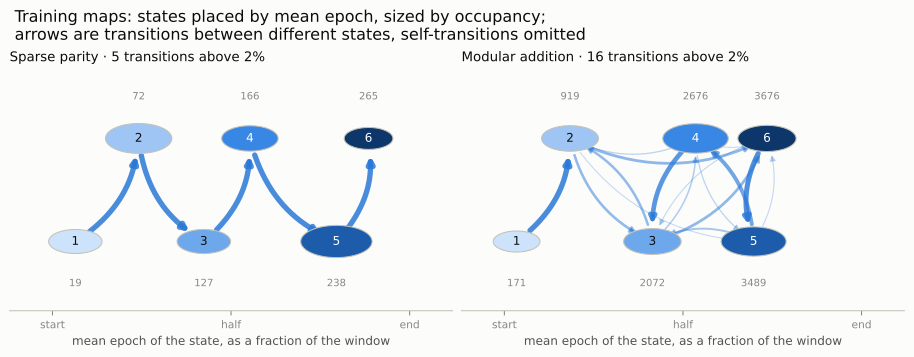
On sparse parities, basically every run goes through the HMM states in the same order. This indicates that the data is essentially one-dimensional. A GMM can easily capture a one-dimensional path.
But on modular addition, the story gets somewhat messier. The HMM is not linear and states get revisited. Let’s look closer.
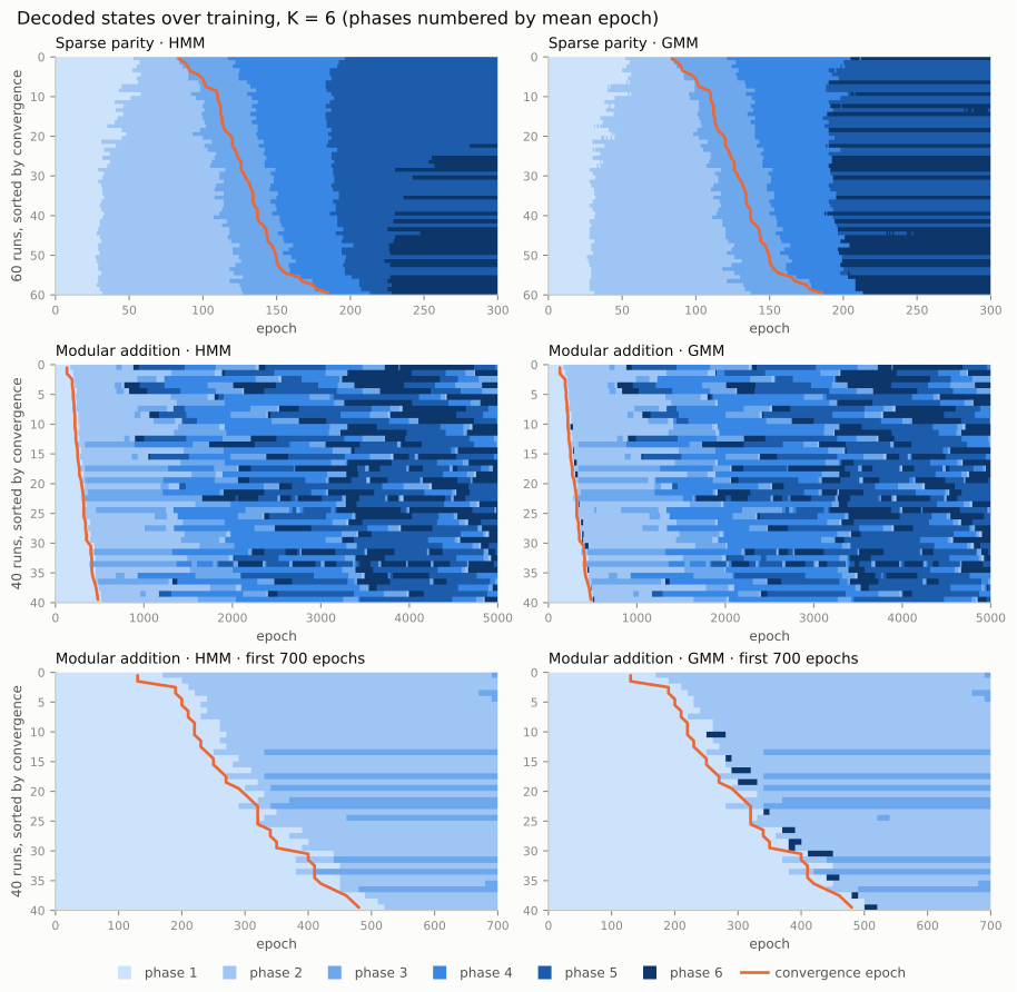
For modular addition, convergence basically tracks with the end of phase 1 in both the HMM and GMM, and phase 1 rarely occurs again. Hence, knowing occupancy for phase 1 (in either the HMM or GMM) lets you read off convergence time.
Comparing against a very naive baseline
What about not even a latent state model?
One alternative is to average all of the 14 weight metrics over the trajectory and then do the regression using the 14 obtained averages. We get the following.
| Task | Evaluation | HMM R² | GMM R² | Averaged metrics R² |
|---|---|---|---|---|
| Sparse parity | Five-fold | 0.968 | 0.965 | 0.957 |
| Modular addition | Five-fold | 0.978 | 0.978 | 0.285 |
It looks like the states are not doing much here, at least for sparse parity. How can we explain this?
Let’s look at the average L1 norm of the weights (entry-wise sum of absolute values). This feature alone gives us an \(R^2\) of \(0.94\).
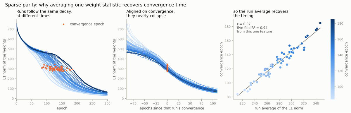
We can see that the runs seem to be basically the same except time-shifted. Moreover, the plots are roughly linear (in the same way the middle of a sigmoid is roughly linear). Note that shifting the x-index (L) by \(k\) should change the average \(L_1\) norm (the area under the curve) by \(k\cdot \alpha\) where \(\alpha\) is some constant. Shifting the x-index also moves the convergence time by \(k\) as every run crosses the convergence threshold at same L1 norm. We then get a linear relationship between the average \(L_1\) norm and the convergence time.
Conclusion
What’s the minimal latent state model for convergence-time prediction? On modular addition, it is a GMM. On sparse parity, it turns out you don’t even need the latent state model. But, a GMM or the 14 averaged features are clearly not good generative models of training dynamics and are unable to capture how training evolves over time. The GMM has no transition structure and the 14 averages are static. Just because they tie with the HMM doesn’t mean that these models capture the dynamics.
So, what are latent state models for training dynamics useful for? At least in this setting, convergence-time regression seems to be a rather weak task to evaluate the HMM model on. Instead, we should target tasks that require the transitions.
Technical Details
| Sparse parity | Modular addition | |
|---|---|---|
| Data | 40-bit inputs, label = parity of the first 3 bits; 1,000 train / 100 test | a + b mod 113; 30% of pairs for training |
| Model | MLP, one hidden layer of width 1,000 | 1-layer transformer, d_model 128, 4 heads, no LayerNorm |
| Optimizer | SGD, lr 0.1, weight decay 0.01, batch 32 | AdamW, lr 1e-3, weight decay 1.0, batch 256 |
| Runs | 60 seeds, trained for this post | 40 seeds, reanalyzed from an earlier cohort |
| Checkpoints | 300, logged every epoch | 500, logged every 10 epochs over 5,000 |
| Convergence epoch | 84–185 (median 129) | 130–480 |
Label: First logged epoch with test accuracy \(\geq 0.9\).
Inputs. Hu et al. (2023)’s 14 weight statistics.
Models. K = 6 states for both, matching Hu et al.’s choice for these tasks
Regression. The features are occupancy which is the fraction of a run’s checkpoints in each state. Features are standardized on the training runs, then fitted with ordinary least squares with an intercept to predict the label.
Main evaluation (five-fold). We do five-fold validation with the runs. Split the runs into five folds; fit the HMM/GMM and the regression on four folds (48 parity / 32 modular runs), then decode states and predict for the held-out fold (12 / 8 runs).
Code
Code can be found here: https://github.com/gaussianprime/latent-state-models-blog-post-code
AI Use Disclosure
Various versions of ChatGPT and Claude Opus were used for help with producing the experiment’s code. They were also used to help brainstorm, draft, outline, format, and proofread this blog post.